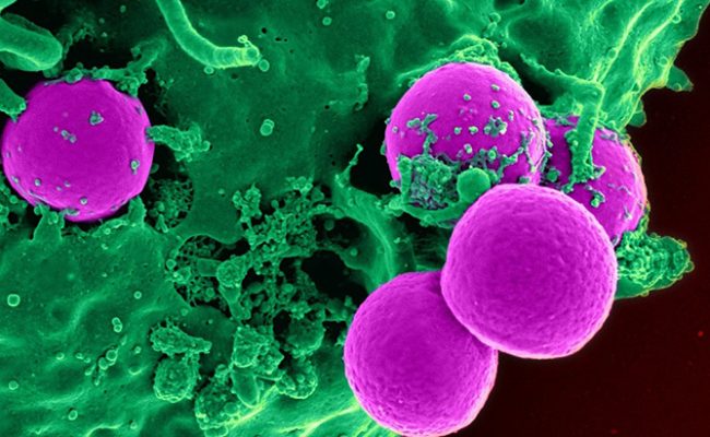
A virus infects by attacking a host cell and using the cell’s support structure to propagate. One way the immune system responds is by deploying cytotoxic T-lymphocytes (CTL) that essentially kill the infected cell and limit the ability of the virus to make copies. The CTL must be able to recognize an infected cell either from prior infection or through the presentation of viral peptides on the surface of the infected cell. Specific drugs can also be administered to disrupt, hinder or halt the mechanism of a virus infecting a host cell and replicating.
The modelling of virus population growth or decay can assist in the characterization of the immune response and in planning drug administration. A basic model is one that has the four sub-populations of numbers of uninfected cells, number of infected cells (the virus load), number of free virus particles and number of CTL. The dynamics of each of these populations is the rate of change of the population due to response to other populations. The number of cells changes because new cells are produced at a characteristic rate and the number of cells that die is proportional to the number of current cells. This is the normal process of the cell life cycle. The number of infected cells changes due to new infections proportional to the number of cells and number of free virus particles. Infected cells also die at a rate that is proportional to the number of infected cells. The number of free virus particles changes as particles are released when the infected cells die through virus induced lysis. Virus ‘death’ is expected to be proportional to the number of virus particles. Finally, the number of CTL changes as it increases in proportion to the number of infected cells and number of current CTL. CTL die at a rate proportional to the number of CTL.
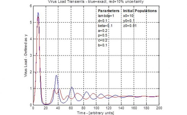
This forms a set of four coupled, first order ordinary differential equations. Simplifications can be applied, seven parameters specified and initial populations specified. Then the equations are solved using numerical integration, such as the 4th-Order-Runge-Kutta method and traditional arithmetic. The result is graphically shown as population numbers versus time. Due to the coupled nature of these equations, there is a cyclic rise and fall of populations such as the infected cells (virus load) and CTL. These cycles define a timing or period between peaks and troughs. Generally the amplitude of the cycles decrease until, after a long time, the population counts reach stable, steady values. Drug administration could use the timing of these curves to take advantage of opportunities such as when virus load is low and is going to be increasing.
Uncertainty in the seven specified parameters, three initial conditions and time are formatted as an 11 dimensional error vector. Then the steps of the 4th-Order-Runge-Kutta method are converted duals arithmetic. This is verified using specified zero error on all errors such that the duals arithmetic becomes exact arithmetic and this should match the traditional arithmetic results. With an error scale control, a 10% error was applied and the resulting virus load curve (see figure for 4th dot) is shown by comparison to the traditional arithmetic curve. This demonstrates the effect of uncertainty as the traditional cycle is disrupted during the second cycle and the remaining curve has its timing changed to be of opposite phase. The uncertainty does not affect the steady state population and both calculations settle around the same time. This result shows that uncertainty might be important to consider when planning treatments that follow a periodic schedule, such as the ‘AIDS cocktail’. The situations and different uncertainties can be tested using the model prior to use in trial experiments.


