
1. About the CertainError Calculator
1.1 CertainError Calculator App
This CertainError Calculator automates error propagation calculations by representing every number as both a value and an error. Traditional arithmetic is replaced by five choices of error propagation arithmetic based on different ways error is geometrically treated. This help menu provides details on each uncertainty arithmetic and operations accomplished by the calculator.
1.2 Authors
The CertainError Calculator was invented by Professor Ronald S. LaFleur of Clarkson University and implemented into app form by Andrew Davis of Jack of Trade Apps located in Potsdam, New York.
2. Using the CertainError Calculator App
2.1.1 Edit boxes
As desired, touch Input X, eX, Input Y, eY to yellow-highlight an edit box. With the numeric touchpad, enter a number in the yellow edit box using decimals where needed.
2.1.2 Angle units
When using trigonometric functions, press RAD or DEG to toggle and choose input angle units. When black DEG appears, the units are in degrees.
2.1.3 Change of sign
When entering numbers in the yellow edit box for X or Y, you can change sign by touching +/- button. The +/- choice does not apply to input of eX or eY as these are treated as unsigned numbers and the +/- is built into the error arithmetic already.
2.1.4 Relative Error
Press RE if the input errors, eX and eY, are relative errors in percent. When a black % appears input errors are in percent. Results are retained as absolute error and use of MX or MY changes the input to absolute error. When black RE appears the inputs are absolute errors.
2.1.5 Backspace
Backspace ![]() edits by deleting from the right to the left
edits by deleting from the right to the left
2.1.6 Clearing
Pressing 'C' clears the contents of the yellow edit box, returning to the default display. Pressing 'C' when no yellow box is present clears all inputs but retains the result.
2.2.1 Binary Operations
Binary operations involve both X and Y and are listed on the right edge of the screen. Touch these and the operation symbol will update between the X and Y inputs. This can be changed any time prior to obtaining answers with a press of the = sign.
2.2.2 Unary Operations
Unary operations are functions with one input. The input X and eX numbers will both be used in the calculation. These functions are listed on the left side grid. Touch these and the operation will appear between the X and Y inputs but the Y inputs will dim as these are not used in Unary operations.
2.2.3 Composite Operations
By using 'result recycling' (see Section 2.4. of this help menu), composite operations and larger algorithms can be accomplished using the fundamental binary and unary operations as building blocks.
For example, a binary operation such as X^Y, where both X and Y have error input, can be completed using a composite formula of R=exp(Y × ln(X)). This composite formula can be converted to a series of steps of unary and binary operations and result recycling using the MX button. See Section 2.3.2. for a numerical example of the X^Y operation.
2.3.1 Results
After inputting numbers, four numbers for binary operations, X, eX, Y and eY, or two numbers for Unary operations, X and eX, and after selecting the operation, touching the = key evaluates every uncertainty arithmetic. The result and its error displayed at the top of the CertainError Calculator screen is selected by choosing the method using the menu to the right. ![]()
The time needed to calculate and display the result depends on the demanding computational time requirements of Monte Carlo (10,000 random instances) and Interval arithmetics (100 instances for one input, 10,000 instances for two inputs). If the calculator did not incorporate these methods, it would be much faster. For example, the Duals arithmetic is very fast by itself.
2.3.2 Unexpected Results
Every number has a center and an error. The center is the conventional interpretation of a number. The error is an extension to the representation. To illustrate, assume the center number is colored white and the error number is colored red.
In the Differential Method (see Section 3 of this help menu), commonly taught at the college level, the center is calculated first, without error(s) so the resulting center is white. This is followed by error calculation that can be a mixture of input center(s) and error(s) so resulting error is pink color.
All other methods either superimpose the input error on the input center (Interval and Monte-Carlo), and these are pink, or assign geometry (chordals and duals). But when the numeric and geometric arithmetic steps are completed, the resulting center can be pink because it could be influenced by the input error(s).
An example of this is X^Y, accomplished with R=exp(Y*ln(X)) and the Duals Method. If X=3, eX=0.1, Y=4 and eY=0.2, then R=78.5121… and eR=20.6408… There is the expectation of R=81 (white) as the Traditional or Differential Methods yield this conventional center value. Then the other methods yield a non-conventional result (pink) and this may be unexpected. Once you appreciate how each method works (see Section 3 of this help menu), you can begin to understand why R is not 81 when X and Y have error.
2.4.1 Results
Most calculations involve many steps. This is managed by organizing a calculation into fundamental Unary and Binary operations with intermediate evaluations and recycling the result by pressing MX or MY. For example, the MX key transfers both the value and the absolute error of the result to the Input X and eX fields with no editing required. If inputs were originally relative error, as percent, using MX or MY transfers the absolute error of the result to the inputs, so the inputs are changed to absolute error.
This essentially converts a result (both center and error) into the X or Y inputs and continued calculation can be performed using the recycled result and/or new inputs for either X or Y. This provides flexibility in completing a calculation. (see Examples 5.2 and 5.4). The downside for some methods is the 'dependency problem.' This occurs when, for example, an X and eX are input (the X error contributes to a result error) and the result is recycled to Y and eY by pressing MY. When the same X and eX are used as inputs again, then the X input error is not independent from the Y error (from recycling). See the section 7 'Glossary' of this Help Menu.
2.5.1 Settings
Current settings are only the sounds issued when buttons are pressed. Choosing an edit box makes a ‘swoosh’ sound. All other sounds are ‘clicks.’ These sounds are active when the ![]() is displayed. Toggle this to turn-off sounds or turn them back on. The volume of the sounds are controlled by the audio settings (loudness and mute) of your device.
is displayed. Toggle this to turn-off sounds or turn them back on. The volume of the sounds are controlled by the audio settings (loudness and mute) of your device.
3. Methods
Methods encompass three things: number representation, arithmetic and rendering of results. Tables are shown to define cases were arithmetic fails (Outlaws) or is permitted (Legals).
3.1.1 About
In Traditional Arithmetic, uncertainty is not calculated because each number remains a single number. The CertainError Calculator app includes Traditional Arithmetic as a choice on the method menu. A number is a geometrically represented as a point on a number line with no error information
![]()
Exact Arithmetic is when zero error is input for any non-traditional method (Intervals, Monte-Carlo, Differentials, Chordals and Duals) and this gives the same answers as Traditional Arithmetic.
3.1.2 | Outlaws and Legals
The CertainError Calculator was invented by Professor Ronald S. LaFleur of Clarkson University and implemented into app form by Andrew Davis of JackOfTradesApps in Potsdam New York.
3.2.1 About Intervals
Intervals are considered a set of points with the error domain populated with a uniform grid of points.
![]()
Calculations are performed by evaluating all combinations of point calculations and then finding the maximum result and the minimum result. The mid-point between the maximum and minimum is the result center and the result error is +/- distance between center and the maximum and minimum.
The number of grid points chosen for each input is important. For example if each input error is grided with 100 points, a calculation with two inputs evaluates 10,000 points and calculation with three inputs evaluates 1,000,000 points. The maximum and minimum are found for the resulting point population.
See these references...
‘A Lucid Interval,’ Hayes, B., American Scientist, Vol. 91, No. 6, November-December, 2003, pp. 484-488.
‘Interval Arithmetic and Automatic Error Analysis in Digital Computing,’ Moore, R.E., Applied Mathematics and Statistics Laboratories, Stanford University, Technical Report No. 25, Nov. 15, 1962, pp. 1-9.
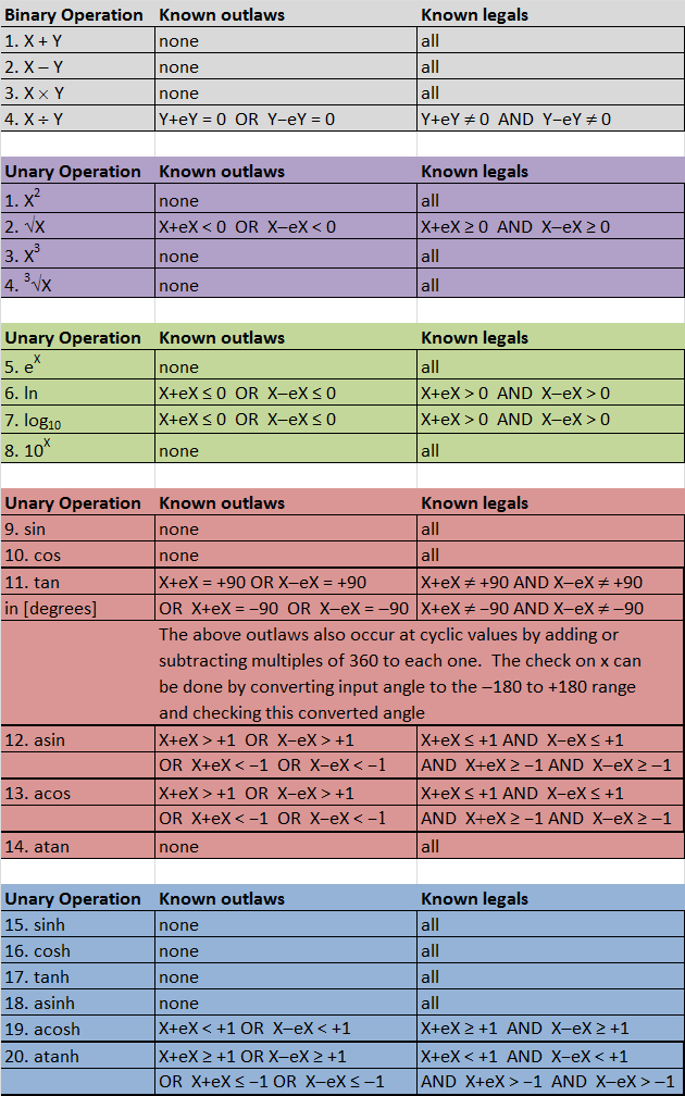
3.2.2 Outlaws and Legals
Outlaws are specific values or range of values that cannot be calculated. Legals are the specific values or range of values the can be calculated. The following table lists them.

3.3.1 About Monte Carlo
The error domain is independently populated with a randomly spaced sample of N points. The size of the random sample, N, is important to obtain stable answers.
![]()
Then each input is a data set of the same size and calculations are done point-by-point. The result data set is of the same size as the inputs. The result center is the mean value of the result data set. The result error is the standard deviation of the data set scaled to a confidence interval using the cumulative student-t distribution (for example 95%) as a coverage factor (1.96 for large N).
See this reference
‘Evaluation of measurement data – Supplement 1 to the “Guide to the expression of uncertainty in measurement” Propagation of distributions using Monte Carlo method,’ JCGM 101:2008. pp. 13-16.
3.3.2 Outlaws and Legals
Outlaws are specific values or range of values that cannot be calculated. Legals are the specific values or range of values the can be calculated. The following table lists them
3.4.1 About Differentials
The center is evaluated first from the error-free inputs (only centers). Knowing the arithmetic operation, a partial differential is formulated for each input and evaluated using the centers. Each of these centered-partial differentials is multiplied by its corresponding error input to get an error contribution. The calculated partial derivatives are only valid within a small range of the center point. This can be a problem if the function is non-linear or has curvature.
![]()
The independent error contributions are combined using a 'Pythagorean Sum,' that is the contributions are squared, the squares are added over inputs and the square root of the total is the resulting error (root-sum-squared, RSS).
See this reference (the differential method dominates in the teaching of engineering)...
‘Describing Uncertainties in Single-Sample Experiments,’ Kline, S.J.; McClintock, F.A., Mechanical Engineering, January 1953, p. 3-8.
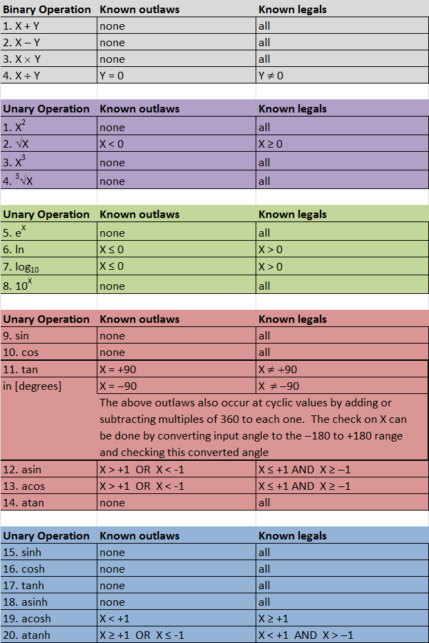
3.4.2 Outlaws and Legals
Outlaws are specific values or range of values that cannot be calculated. Legals are the specific values or range of values the can be calculated. The following table lists them.
3.5.1 About Chordals
An upper point for each input is obtained by adding the error to each center. Similarly, a lower point is obtained by subtracting the error from each center. A chordal is a shortest-distance line segment spanning two extreme points, therefore only the points are important
![]()
The input to each calculation step is coordinated by a signature of (+1,-1) to how it determines the upper or lower points for the result. For example, if subtraction is used, C=C1-C2, the upper point of the result C is determined by the upper point of C1 and the lower point of C2. This typically gives the worst case error as the calculation is based on the bounds of error domains and the arithmetic is performed on a ‘flat’ geometry of scaled points. Implementation is made difficult when inputs appear more than once in a calculation step and sensitivity of output to inputs is cloudy.
One unpublished reference (patents pending)
Lecture 9 – Chordals,’ ES581 Fall 2014 Course Notes, Prof. R.S. LaFleur
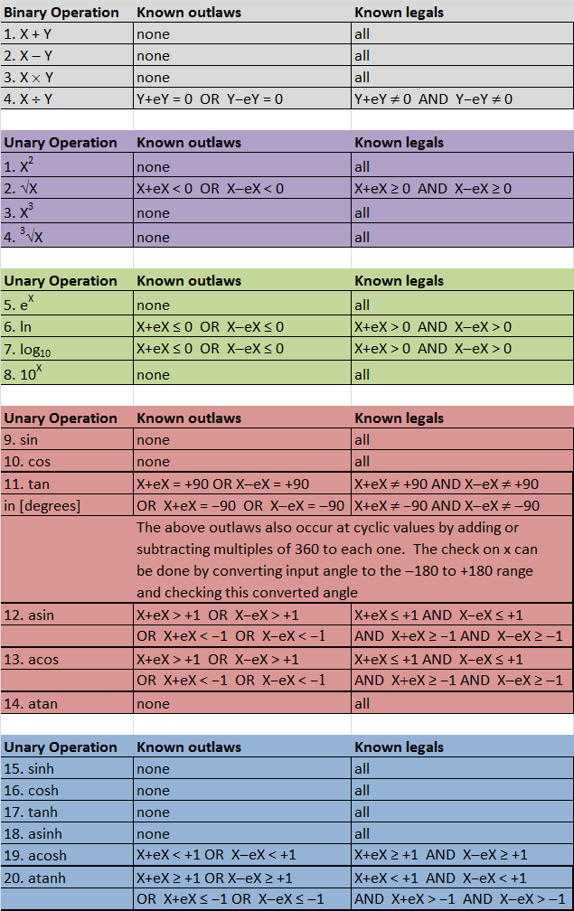
3.5.2 Outlaws and Legals
Outlaws are specific values or range of values that cannot be calculated. Legals are the specific values or range of values the can be calculated. The following table lists them
3.6.1 About the Duals Method
A dual is a geometry that has a simultaneous point and error vector. The error vector simultaneously has two directions
![]()
The error for every quantity has dimension equal to the number of inputs. For example, a binary operation has two inputs so the error vector of both inputs is two-dimensional. Unary functions have one input so the error vector is one-dimensional. This format is used consistently for every operation and through the entire calculation procedure so the result has the same format. A 'Dual' is a number with a 1D error vector. 'Duals' are numbers that have multi-dimensional error vectors.
One unpublished reference (patents pending)...
‘Lecture 16 – 2D Applications,’ ES581 Fall 2014 Course Notes, Prof. R.S. LaFleur
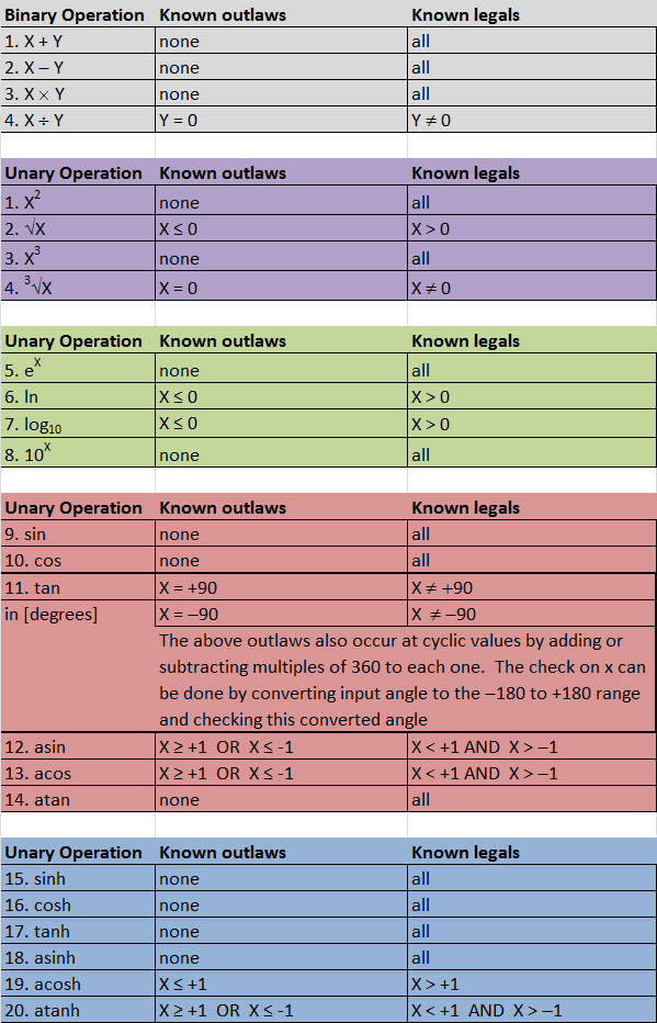
3.6.2 Outlaws and Legals
Outlaws are specific values or range of values that cannot be calculated. Legals are the specific values or range of values the can be calculated. The following table lists them
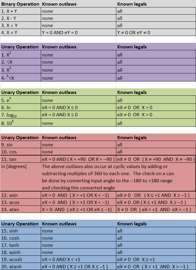
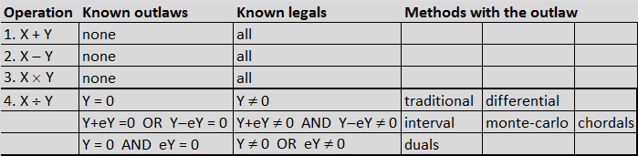
4 | Operations
4.1.1 About Binary Operations
Binary operations involve both X and Y and are listed on the right edge of the screen. Touch these and the operation symbol will update between the X and Y inputs. This can be changed any time before you press = to get results. The common binary operations are the traditional arithmetic of addition, subtraction, multiplication and division. When number representations are changed to include simultaneous error, the arithmetic is expanded to allow simultaneous error calculation.
4.1.2 Outlaws and Legals
Outlaws are specific values or range of values that cannot be calculated. Legals are the specific values or range of values the can be calculated. The following table lists them
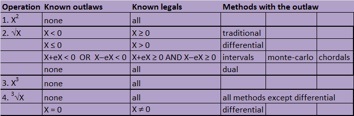
4.2.1 Powers and Roots
4.2.1.1 About Powers and Roots
Powers are when a number is raised to an exponent of an exact integer such as squaring and cubing. Roots are the opposite of powers as the exponent is an exact fraction such as 1/2 for square root and 1/3 for cube root. While traditional software reports one answer, such as the square root, it is common knowledge that the result is two answers, both the + and the – of the square root. On top of this is the bipolar (±) error. When multiple roots exist, they are all calculated and each has an error number. The result reported by the CertainError Calculator is the root with the least error.
4.2.1.2 Outlaws and Illegals for Powers and Roots
Outlaws are specific values or range of values that cannot be calculated. Legals are the specific values or range of values the can be calculated. The following table lists them
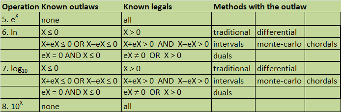
4.2.2 Exponentials and Logarithms
4.2.2.1 About Exponentials and Logarithms
Exponential functions have common use in growth or decay models and in compound probability. Logarithms are commonly used to discover non-integer exponents or to scale data prior to regression. The exponential and logarithm functions are inverses and are paired. The CertainError Calculator includes base-10 and the natural base of e=2.7182… Other bases can be completed by scaling (by multiplying by an exact constant) to either of these two bases using well-known formula. Using this approach, the arbitrarily chosen base can also be formatted with error.
4.2.2.2 Outlaws and Legals for Exponentials and Logarithms
4.2.3 Trigonometry
4.2.3.1 About Trigonometry
The sine, cosine and tangent functions are common operations on scientific calculators. The CertainError Calculator includes these with error formatted and calculated according to each of the uncertainty arithmetics. The user has the option of choosing the units of X by pressing DEG or RAD. Other trigonometric functions such a secant, cosecant or cotangent are obtained by taking the appropriate reciprocal of the sine, cosine or tangent results. The reciprocal is obtained by using the MY button to send the result to the input Y fields, inputting exact 1 for X and choosing the divide operator (see Examples: Reciprocal and trigonometry).
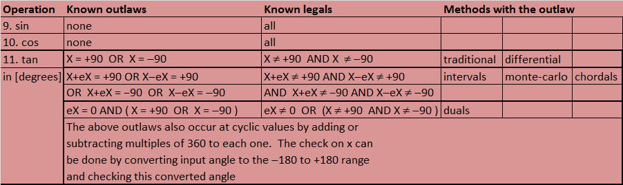
4.2.3.2 Outlaws and Illegals for Trigonometry
Outlaws are specific values or range of values that cannot be calculated. Legals are the specific values or range of values the can be calculated. The following table lists them
4.2.4 Hyperbolics
4.2.4.1 About Hyperbolics
Hyperbolic functions are common operations on scientific calculators. The CertainError Calculator includes these with error formatted and calculated according to each of the uncertainty arithmetics.
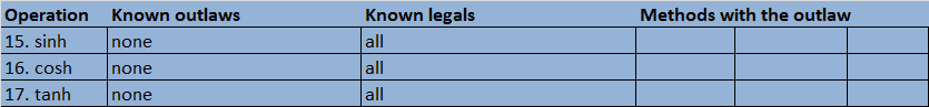
4.2.4.2 Outlaws and Illegals for Hyperbolics
Outlaws are specific values or range of values that cannot be calculated. Legals are the specific values or range of values the can be calculated. The following table lists them
4.3.1 Inverse Trigonometry
4.3.1.1 About Inverse Trigonometry
The inverse sine, cosine and tangent functions are common operations on scientific calculators and are paired with the sine, cosine and tangent functions by toggling the INV key. The CertainError Calculator includes these with error formatted and calculated according to each of the uncertainty arithmetic. The units of the results can be selected by toggling the DEG or RAD key.
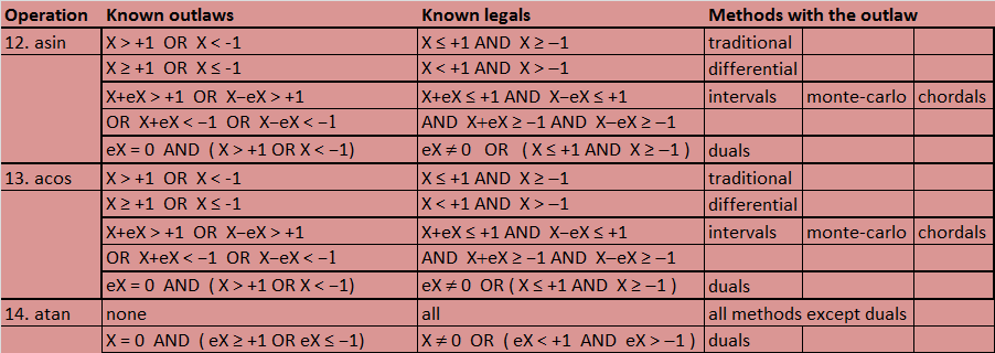
4.3.1.2 Outlaws and Illegals for Inverse Trigonometry
Outlaws are specific values or range of values that cannot be calculated. Legals are the specific values or range of values the can be calculated. The following table lists them
4.3.2 Inverse Hyperbolics
4.3.2.1 About Inverse Hyperbolics
Inverse hyperbolic functions are common operations on scientific calculators and are paired with the sinh, cosh and tanh functions by toggling the INV key. The CertainError Calculator includes these with error formatted and calculated according to each of the uncertainty arithmetics.
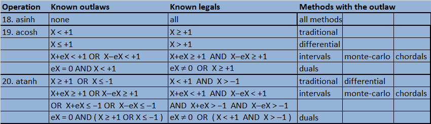
4.3.2.2 Outlaws and Legals for Inverse Hyperbolics
Outlaws are specific values or range of values that cannot be calculated. Legals are the specific values or range of values the can be calculated. The following table lists them
5 | Examples using the CertainError Calculator
Multiplication Example using the CertainError Calculator
- Input X = 68.9
- Input eX = 0.05
- Input Y = 25.3
- Input eY = 0.05
- Choose operation: X (multiplication)
- Press: = (equal)
The answers are (rounding to the error level), by using the method menu to view results
| # | Title |
|---|---|
| Traditional | 1743 ± 0 cm2 |
| Intervals | 1743 ± 4.71 cm2 |
| Monte Carlo | 1743 ± 4.15 cm2 |
| Differential | 1743 ± 3.67 cm2 |
| Chordals | 1743 ± 4.71 cm2 |
| Duals | 1743 ± 3.67 cm2 |
Calculate the cosecant of 75 degrees with an error of 2.5 degrees. This is accomplished by the following steps:
- Choose the uncertainty arithmetic as Differential
- Press RAD to change to DEG units
- Input X 75
- Input eX 2.5
- Choose operation: sine or sin
- Press =
- Press MY
- Clear X
- Input X 1
- Clear eX
- Input eX 0
- Choose operation: +
- Press: =
The result is (with rounding): 1.035 ± 0.0121
A stock was purchased for $300 per share over a day with 1% relative volatility. A year later, the stock shares were sold at $400 per share over a day with 1% relative volatility. What is the capital gain and the volatility of the capital gain in dollars? This is solved using the following steps
- Choose uncertainty arithmetic as Monte Carlo
- Input X = 400
- Press RE
- Input eX = 1
- Input Y = 300
- Input eY = 1
- Choose operation - (minus)
- Press = (equals)
- The answer (with rounding) is $100.00 ± $5.69 (this may vary due to random sampling)
- Press =
- Press =
- Press =
- Change the method to duals and new results are displayed as $100.00 ± $5.00
For example, a cell culture grows by cell division with the following equation and numbers

This is organized into a sequence of 26 steps on the uncertainty calculator, following the equivalent formula

- Choose uncertainty arithmetic to be used through the calculation

- Input X 2
- Input eX 0
- Choose operation ln
- Press =
- Press MX
- Choose operation / (divide)
- Input Y 2.5
- Input eY 0.4
- Press =
- Press MX
- Choose operation ´
- Clear Y
- Input Y 6
- Clear eY
- Input eY 0
- Press =
- Press MX
- Choose operation eX
- Press =
- Press MX
- Choose operation X (multiply)
- Clear Y
- Input Y 200
- Clear eY
- Input eY 25
The answer for the cell count, rounded to whole numbers is N = 979 ± 287
6 | Beyond the CertainError Calculator
The CertainError Calculator app is an extension of traditional calculators. This provides easier uncertainty and error analysis by automating the arithmetic of the most common functions found on college-level scientific calculators. However, there are limitations to the calculations to make it feasible to operate on a hand-held device and in short time.
For example, the Monte Carlo method used in the CertainError Calculator uses a population of 10,000 random samples. This is large enough to demonstrate the calculator’s capability but the stability of the answers could be improved by using a much large random sample, for example, 1,000,000. This large a sample is commonplace in financial and other applications. Larger sample sizes can be easily implement on computer platforms using CertainError software.
Another limitation is that the interval method is implemented using a grid of 100 points per input. This means the unary functions have a population of 100 points and the binary functions have a population of 10,000 points. This suffices to capture a good representative maximum and minimum. A higher density grid would provide a higher resolution on the answer and this might be important with functions that have rapid changes occurring. Increasing the number of inputs greatly increases the required number of evaluation points. These demands are easily met using computer hardware and CertainError software.
If a calculation uses an input quantity more than once, then the dependency problem occurs (see the glossary for a definition). The duals method is the only arithmetic that solves the dependency problem, keeping error contributions of each input independent through the calculation. A larger number of inputs require that the duals arithmetic be formatted to larger dimension error vectors. The CertainError Calculator has a maximum of two inputs and this works as long as a number is not input more than once. If a calculation does have an input used more than once, it is better to implement the duals arithmetic on a computer using CertainError software products.
7 | Glossary
Error is a number that communicates the difference between a true value and a quantized value. The quantized value is a number either from a measurement scale (source error) or the result of a calculation (propagated error). The true value is usually unknown, thus providing the motivation for measurement. The true value can also be a specified target a system attempts to achieve. When the true value is unknown, the error cannot be known. However the error is bounded by the resolution of the quantized value so ‘error’ is interpreted as error limits. When dealing with measurements, a physical instance is rounded to one point on the measurement scale. Nearest rounding produces a bipolar error source (+/-). When dealing with calculations, propagated error is typically bipolar because it inherits the +/- from a square root operation. Error is fundamental to every number and does not involve populations, statistics, distributions or expected value theory. The geometry of the error depends on the chosen uncertainty arithmetic.
Uncertainty is the accumulation of error instances into a population and using statistics to assign an error number. A source error is often a pre-calculation of input sample data using standard deviation and the student-t sample distribution that sizes the error ‘bar’ according to a desired level of confidence or probability. If the student-t value is not explicitly used, it is essentially t=±1, and this captures only between 50% (N=2) and 68.3% (N=1,000,000) of the data.
Uncertainty is a broader term than error because uncertainty involves both source errors and deviations and can consider probability. Since formulas are used to calculate, uncertainty is really a propagated error but it is augmented by deviations. Note that standard deviation cannot be calculated for a sample that has only one measurement (N=1) but error still remains on that measurement. The geometry of uncertainty is a triangle and is a right triangle when errors are independent from deviations.
This is a term used in traditional statistics to describe the standard-deviation-of-the-mean. An original one-sample of data has one mean value and one standard deviation. Ten samples result in ten mean values and ten standard deviations. One-hundred samples result in one-hundred mean values and standard deviations. Then, on that level, there is a sample population of mean values. This sample of means also has statistical measures such as a mean value and a standard deviation. This can be called mean-of-the-mean and standard-deviation-of-the-mean. Applying theory, the standard-deviation-of-the-mean or ‘standard-error’ is calculated from an average standard deviation and the size of the original one-sample. Total errors scale as the square-root of the sample size while deviations scale as the square-root of the sample size minus one.
Therefore, although ‘standard error’ is calculated from deviations, it is called error to be consistent with the sample size scaling. Since 'Standard Error' is based on standard deviation, it can not be calculated for samples that have only one instance (N=1), thus it is really not an error but it is a type of deviation.
Traditional arithmetic of addition, subtraction, multiplication and division is between two numbers. In a process diagram, this appears as two inputs into a process and one output result. The binary operation symbol is placed between X and Y. X is called an ‘object’ and Y is called a ‘subject.’ The binary operation symbol combined with the subject defines a modifier that acts upon the object to create a result. With addition and subtraction, the result is called a resultant. With multiplication and division, the result is called a product.
Many traditional functions involve only one number, X. On a process diagram, this appears as one input into a process and one output result. The function format is a function name and parentheses that enclose the X input, such as sin(X) for the sinusoidal function. Inverse Unary functions are the same format as Unary functions.
When a multiple-step calculation uses an input quantity and its error more than once, this creates something called ‘the dependency problem.’ This is due to error propagation arithmetic assuming inputs to calculation steps are independent. While this is true for the unary and binary operations of the CertainError Calculator, it is not true when using the calculator to accomplish a larger calculation. The first-use of an input inserts its error contribution to the first-result; the result depends on that input. A second-use of that input inserts its error contribution again but this is not independent because the first-result carries an error contribution from the first-use. So the dependency problem is seen for multiple calculation steps when an input’s information has more than one path.
Sometimes the algorithm can be reoriented so that each input has only one path and the error contributes once. But this is a challenge and not always possible to complete. The Duals arithmetic is the best way to implement such a calculation using a computer and software. However, multiple input calculations, such as totaling instances over a sample or mean value of a sample, can be calculated using the CertainError Calculator by repeated recycling of intermediate results using the MX button.
The dependency problem can be shown by an example of simple arithmetic. This is the calculation of a quantity, R, from two algebraically equivalent formula shown below.
Version 1 Two Operations R1 = c*(a ‒ b)
Version 2 Three Operations R2 = (c*a) ‒ (c*b)
Version 2 has the ‘c’ contributing in two places or on two calculation paths and this requires writing down an intermediate answer for later input. The dependency problem is when results for these two versions do not match, either by the center values or by the error. Answers for R, R1 and R2, must match completely (both centers and errors) to successfully avoid the dependency problem.
Each version should be calculated for each choice of uncertainty arithmetic. Two recipes using the CertainError Calculator are shown below.
Version 1
- Input X (this is ‘a’ in the formula) 3
- Input eX 0.3
- Input Y (this is ‘b’ in the formula) 2
- Input eY 0.2
- Choose operation as minus or -
- Press =
- Press MY
- Clear X
- Input X (this is ‘c’ in the formula) 5
- Clear eX
- Input eX 0.5
- Choose operation as multiply or ´
- Press = to get result R1
- For the uncertainty arithmetic chosen, write the R1 results in the table
Version 2
- Input X (this is ‘c’ in the formula) 5
- Input eX 0.5
- Input Y (this is ‘a’ in the formula) 3
- Input eY 0.3
- Choose operation as multiply or ´
- Press =
- Write down the center and error of the intermediate answer (c*a)
- Clear Y
- Input Y (this is ‘b’ in the formula) 2
- Clear eY
- Input eY 0.2
- Choose operation as multiply or ´
- Press =
- Press MY
- Clear X
- Input X (this is the center of the intermediate answer)
- Clear eX
- Input eX (this is the error of the intermediate answer)
- Choose operation as minus or ‒
- Press = to get result R2
- For the uncertainty arithmetic chosen, write the R2 results in the table
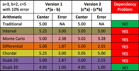
As expected, the traditional arithmetic does not have a dependency problem because it does not provide any uncertainty information.
For this simple example, the Interval and Chordal arithmetic match and the centers of the Duals arithmetic (2D) and Differential arithmetic match. The (YES) dependency problem means you have to be careful when implementing arithmetic to calculate larger problems as the answers will differ. This is a practical constraint on uncertainty calculations.
The Duals arithmetic used on the CertainError Calculator app has the dependency problem because the calculator is formatted for binary operations with independent errors input. The Duals 3D arithmetic implemented on a computer using CertainError software uses the full 3D format for all numbers (a,b,c) and provides the only solution to this dependency problem.
The Duals arithmetic implemented in software is the only method that solves the dependency problem for any number of inputs (dimensions, D), from 2D, 3D and 4D up to any dimension, nD. This makes implementation of simple arithmetic operations to perform larger calculations very flexible as the user can decide to use any arrangement of calculation steps. Later versions of the CertainError Calculator are planned to allow any dimension of inputs.